import matplotlib.pyplot as plt
import yaml
import numpy as np
from ruspy.simulation.simulation import simulate
from ruspy.model_code.fix_point_alg import calc_fixp
from ruspy.model_code.cost_functions import lin_cost
from ruspy.model_code.cost_functions import calc_obs_costs
from ruspy.estimation.estimation_transitions import create_transition_matrix

Simulation tutorial

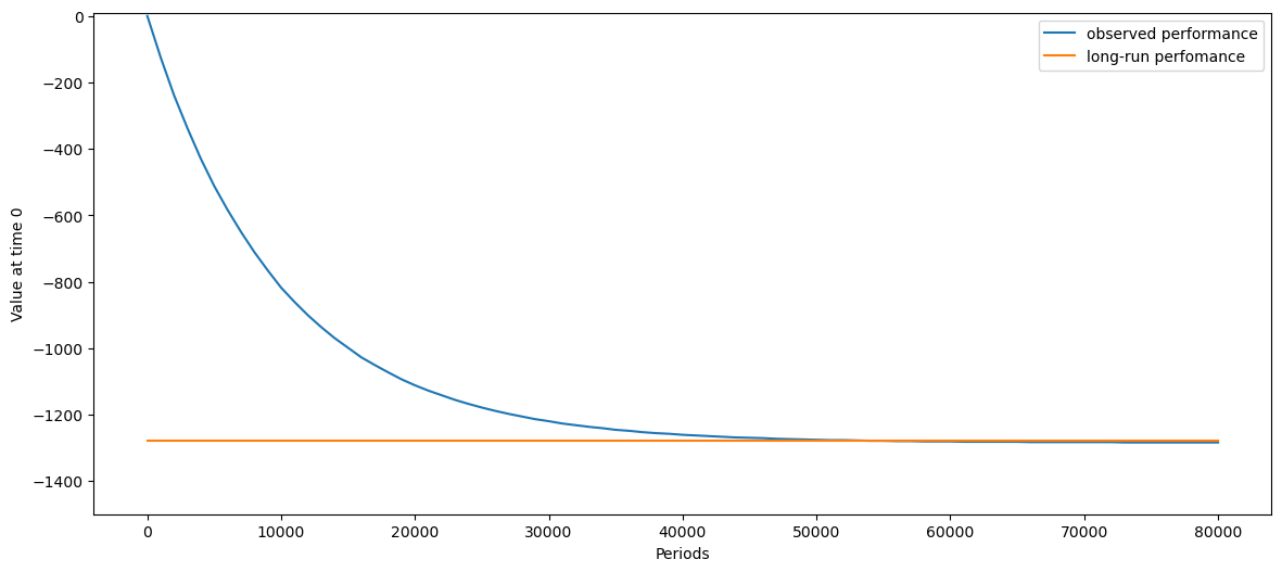
This notebook provides a tutorial of how to use ruspy’s simulation function simulate. Furthermore, the convergence of expected utility calculated by fixed point algorithm and the observed utility on the simulated data are demonstrated.

First we specify the initialization dictionairy for the simulation.

# Set simulating variables
disc_fac = 0.9999
num_buses = 100
num_periods = 80000
gridsize = 1000
# We use the cost parameters and transition probabilities from the replication
params = np.array([10.07780762, 2.29417622])
trans_probs = np.array([0.39189182, 0.59529371, 0.01281447])
scale = 1e-3

init_dict = {
    "simulation": {
        "discount_factor": disc_fac,
        "periods": num_periods,
        "seed": 123,
        "buses": num_buses,
    },
    "plot": {"gridsize": gridsize},
}

Beside the initializsation dictionary, the simulate function takes other inputs. These objects are calculated below and are passed to the simulation function, which returns the simulated data.

# Calculate objects necessary for the simulation process. See documentation for details.
num_states = 200
costs = calc_obs_costs(num_states, lin_cost, params, scale)

trans_mat = create_transition_matrix(num_states, trans_probs)
ev = calc_fixp(trans_mat, costs, disc_fac)[0]

# Simulate the data.
df = simulate(init_dict["simulation"], ev, costs, trans_mat)

In the following, a exercise is provided, which shows the convergence of expected utility calculated by fixed point algorithm and the observed utility on the simulated data.

# Provide a discounting function.
def discount_utility(df, disc_fac):
    v = ((disc_fac ** df.index.get_level_values("period")) * df["utilities"]).sum()
    return v / df.index.get_level_values("Bus_ID").nunique()

# Discount the utility of the observed data
num_points = int(num_periods / gridsize) + 1

periods = np.arange(0, num_periods + gridsize, gridsize)

v_disc = np.zeros_like(periods)
for i, period in enumerate(periods[1:]):
    v_disc[i + 1] = discount_utility(df[df.index.get_level_values("period") <= period], disc_fac)

# Create an array containing the expected long-run performance.
v_exp = np.full(num_points, ev[0])

The results are now visualized in oder to show convergence of the observed utility on the simulated data to the expected utility by the fixed point algorithm.

fig, ax = plt.subplots(figsize=(14, 6))

ax.set_ylim([-1500, 10])

ax.set_ylabel(r"Value at time 0")
ax.set_xlabel(r"Periods")

ax.plot(periods, v_disc, color="#1f77b4", label="observed performance")
ax.plot(periods, v_exp, color="#ff7f0e", label="long-run perfomance")

ax.legend()

<matplotlib.legend.Legend at 0x7fce11936b20>